Research Topics
Tools: Moment tensor inversion and earthquake relocation
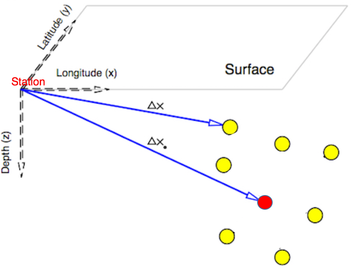
Earthquake relocation and source study are two powerful tools to investigate the style of deformation in different tectonic settings. Figure below shows a simple illustration of these techniques.
Earthquake relocation and source study are two powerful tools to investigate the style of deformation in different tectonic settings. Figure below shows a simple illustration of these techniques.
|
|
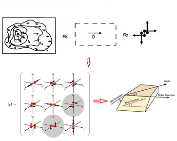
Left panel: a simplified cartoon showing the main idea behind relocation methods. Despite single event location, a cluster of earthquakes can be located together to reduce the contribution of error imposed by the imprecise velocity model. Right panel: a space-time history of the slipping motion on a fault can be approximated by a double-couple force modeling. Based on this approximation, we resolve moment tensor elements that are related to the strike, the dip, and the rake of a fault (Aki and Richards, 2002).
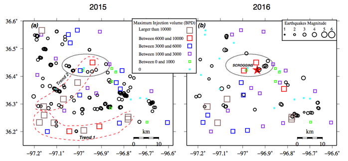
Figure below compares the single event location from the IRIS catalog with results of relocation of earthquake clusters in the Pawnee region, Oklahoma. We applied a source-specific station term method and a differential time relocation method based on waveform cross correlation (Lin and Shearer., 2005; Lin and Shearer., 2006; Lin et. al., 2007).
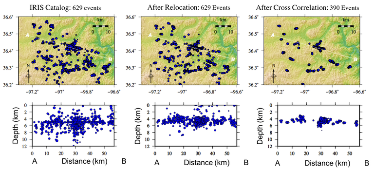
The relocation results has improved the spatial distribution of earthquakes both in the map view and at depth.
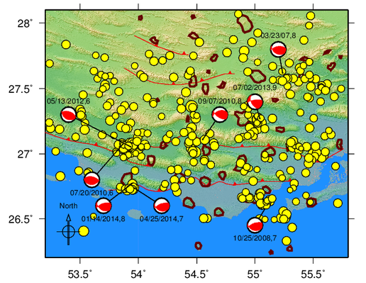
Below is an example of the moment tensor inversion and the testing of stability of the solution for an earthquake in the Zagros, Iran (Aziz Zanjani and Ghods, 2015).
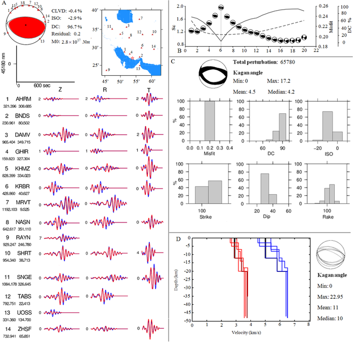
The representation of the moment tensor inversion and the stability of our solution for the earthquake (07/20/2010) in frequencies between 0.17 and 0.04 Hz (Aziz Zanjani and Ghods, 2015). We used mtinvers program (Dahm and Kruger, 1999; Donner et. al, 2013) for moment tensor inversion. A) Blue and red lines are observations and synthetics, respectively. The number beside each waveform is the value of the time shift. The number below the name of each station represents the focal distance and the azimuth of the station from the epicenter, respectively. B) The solution at different depths. Beach balls are showing the DC part of solutions. Dotted lines show the misfit between the observation and the synthetics. The solid line shows the SC value at each depth (the Sc value represents the depth with a minimum misfit and a maximum DC). The grey line specifies the centroid depth. C) The Jacknife test and the corresponding Kagan angle. D) (left) Different velocity models for S and P waves (the red line for the P wave and the blue line for the S wave), black solid lines show the selected velocity models. (right) Solutions for different velocity models and their related Kagan angles .